Wastewater Treatment Plant Design...
Chapter 02 - Preliminary Treatment...
2.1. Introduction...
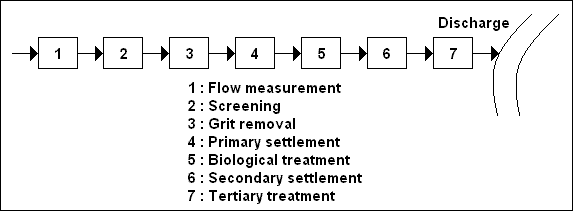
The inflow to a sewage works is dependent on the sewerage system. In a totally separate system where the minimum amounts
of surface water are taken to the sewage works, the total inflow may receive the type of treatment shown diagrammatically
in figure given below.
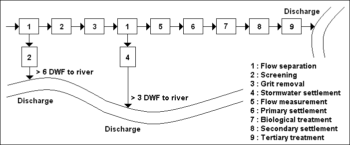
In some parts of the world it has been common to give up to 3 times dry weather flow, preliminary, primary and secondary
treatment while flows above 3 DWF are treated as shown in figure given below.
The method used to define the value of 3 DWF and 6 DWF has varied, but a modern definition is ;
3 DWF = 3 NG + I + 3 E
6 DWF = NG + I + 1,360 N + 3 E
where ; N : population, G : unit water usage ( L / capita . day ), I : total infiltration flow to the sewers in dry
weather ( L / day ) and E : total dry weather industrial flow ( L / day ). DWF is defined as the flow in the sewer
over 24 h when no rain has fallen for several days.
Preliminary treatment includes flow measurement, flow separation, screening and communition of solids, removal
of grit, and sedimentation.
2.2. Flow Measurement...
 For more info about the "Flow Measurement"...
Measurement of flows is a major consideration in sewage treatment. In general, V notch and rectangular thin plate
weirs are more suitable for influent and effluent measurement.
V - Notch Weirs...
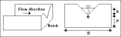
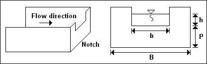
The general expression for the flow Q ( m 3 / s ) over a V - notch weir of the type shown in figure given
below ;
Q = ( C ) ( h ) 5 / 2
where ; h : the vertical head through the notch measured from the "vertex" of the notch to the TWL, which in turn is
measured a distance of 3 to 4 times the maximum head, upstream of the weir. C is a constant which includes a term for
the velocity of approach and is numerically equal to ;
C = ( 1.40 ) Tan ( THETA / 2 )
Approach velocity term ( V ) 2 / ( 2 g ) should be less than h.
Another V - notch equation is ;
Q = ( 8 / 15 ) ( MU ) Tan ( THETA / 2 ) ( 2 g ) 1 / 2 ( h ) 5 / 2
MU = 0.565 + 0.0087 / ( h ) 1 / 2
Example 2-1 :
Determine the flow range within which a 90 O V - notch weir may be used according to BS - 3,680 for a 1 m
wide channel.
Calculation :
( h / B ) <= 0.20, i.e. h <= 0.20 m and B = 1.00 m
( h / P ) <= 0.40, i.e. for the minimum value of P of 0.45 m
h <= 0.18 m
Thus by increasing P to 0.50 m the raito of ( h / B ) becomes the limiting criterion for maximum flow. A minimum value
for h of 0.05 m is required. Thus ;
Q MIN = ( 1.40 ) ( 0.05 ) 5 / 2 = 0.0008 m 3 / s = 0.8 L / s
Q MAX = ( 1.40 ) ( 0.20 ) 5 / 2 = 0.025 m 3 / s = 25 L / s
It should be noted that under maximum flow conditions the upstream velocity is ;
( Q MAX ) / [ ( B ) ( P + h ) ] = ( 0.025 ) / [ ( 1.00 ) ( 0.50 + 0.20 ) ] = 0.036 m / s
and an approach velocity term ( V ) 2 / ( 2 g ) would be 6.5 x 10 - 5 m which is negligible
compared with a value for h of 0.20 m.
Rectangular Weirs...
( a ) Full width or suppressed weirs : These run the full width of the channel and consequently the nappe is not
fully aerated. BS - 3,680 suggests the use of the "Rehbock" equation although others exist, i.e. ;
Q = ( 2.95 ) ( B ) [ 0.602 + ( 0.083 ) ( h / P ) ] ( h + 0.0012 ) 3 / 2
The operational restrictions are that ( h / P ) <= 1.00, 0.03 m < h < 0.75 m, B >= 0.30 m and P >= 0.10 m.
Example 2-2 :
A full width thin plate rectangular weir is to be used in a 0.40 m wide channel, P being 0.20 m. Calculate the maximum
allowable flow.
Calculation :
Since ( h / P ) <= 1, then h <= 0.20 m ( i.e. this is within the range 0.03 - 0.75 m ). Therefore ;
Q = ( 2.95 ) ( 0.40 ) [ 0.602 + ( 0.083 ) ( 1 ) ] ( 0.20 + 0.0012 ) 3 / 2 = 0.073 m 3 / s
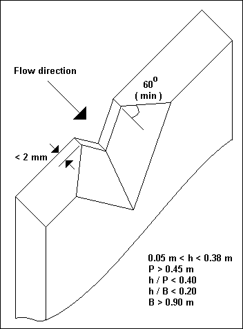
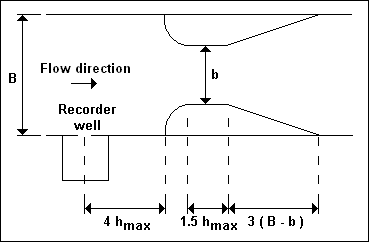
( b ) Partial width weirs : A primary requirement is that the approach channel width shall be > ( 4 h + b )
where h and b are is in figure given below.
- ( B - b ) / 2 > 2 h
- P >= 2 h MAX
- ( h / b ) <= 0.50
- 0.08 < h < 0.60
- P > 0.30 m
- b > 0.30 m
Under these conditions the contractions are fully developed and the expression relating discharge to head is ;
Q = ( 1.82 ) [ 1 - ( 0.10 ) ( h / b ) ] ( b ) ( h ) 3 / 2
Example 2-3 :
Assuming a weir of minimum width 0.30 m, determine the head h and hence the channel width for a flow of 0.037
m 3 / s
Q = 0.037 = ( 1.82 ) ( 0.30 - 0.10 h ) ( h ) 3 / 2
h = 0.166 m
Using this in the expression ( 0.30 - 0.10 h ) ( h ) 3 / 2 , gives 0.0192 and hence Q = 0.035. However,
it is obvious that ( h / b ) exceeds 0.50, therefore the weir must be extended. Therefore, try b = 0.40, hence ;
( 0.037 / 1.82 ) = ( 0.40 - 0.10 h ) ( h ) 3 / 2
And assuming 0.10 h to be small ;
h = [ 0.037 / ( 1.82 x 0.40 ) ] 2 / 3 = 0.137 m
Trying h = 0.14 m gives ;
( 1.82 ) ( 0.40 - 0.10 x 0.14 ) ( 0.14 ) 3 / 2 = 0.037 m 3 / s
i.e. this the correct solution. The walls must be 2 h away from the weir sides, thus B = 4 h + b or 0.96 m ; compare
this channel width with that in Example 2-2.
Flumes...
A commonmethod of measuring flows containing gross solids ( which would settle out if a weir were used ), is a standing
weve flume.
Q = ( 1.71 ) ( b ) ( h ) 3 / 2
where ; b : throat width, h : depth of flow through the flume, measured a distance of 4 h MAX upstream.
2.3. Flow Separation...
In many instances some form of flow separation is required. The excess is transferred to stormwater settlement tanks.
One method is to use side weirs that are controlled by a downstream standing wave flume as below.
Example 2-4 :
A sewage works is designed for a future population ( N ) of 10,000 persons with a daily water usage ( G ) of 230
L / capita. Industrial effluent ( E ) and the infiltration ( I ) will be neglected. Estimate the dimensions of a
broad crested side weir ( controlled downstream by a standing wave flume ) used to separate flows between 3 DWF and
maximum stormwater flow Q MAX ( 6 DWF ).
Calculation :
- 3 DWF = ( 3 ) ( N ) ( G ) = ( 3 ) ( 10,000 ) ( 230 ) = 6,900,000 L / day = 6,900 m 3 / day = 0.08
m 3 / s
- Q MAX = ( N ) ( G ) + ( 1,360 N ) = ( 10,000 ) ( 230 ) + ( 1,360 x 10,000 ) = 15,900,000 L / day =
15,900 m 3 / day = 0.18 m 3 / s
The difference is 0.10 m 3 / s. The formula for a broad crested weir is ;
Q = ( 1.71 ) ( W S ) ( h S ) 3 / 2
where ; W S : the side weir width ( m ) and h S : the side weir head ( m ). For this calculation
using a double sided weir ;
W S = ( 1 / 2 ) { ( 0.10 ) / [ ( 1.71 ) ( h S ) 3 / 2 ] }
Ideally, the side weir should be capable of spilling the difference between Q MAX and 3 DWF while keeping
the same maximum head, h MAX , through the flume, where h MAX corresponds to 3 DWF. In practice
the difference in head in the flume for flows upstream of Q MAX and 3 DWF will vary by the maximum head
over the side weir h S , thus h should be kept low, e.g. 0.05 m. Therefore ;
W S = ( 1 / 2 ) { ( 0.10 ) / [ ( 1.71 ) ( 0.0112 ) ] } = 2.6 m each side
If a width for the flume of say 0.30 m has previously been calculated, the crest of the side weir would be above the
channel invert by the value of the flume head at 3 DWF, i.e. ;
h = { ( 0.08 ) / [ ( 1.71 ) ( 0.30 ) ] } 2 / 3 = 0.290 m
At maximum flow the flume would actually be operating with a head of 0.290 + 0.05 = 0.340 m ; equivalent to a flow of
( 0.30 ) ( 1.71 ) ( 0.340 ) 3 / 2 or 0.10 m 3 / s, i.e. 3.8 DWF. Increasing the flow through the
works to 3.8 DWF would greatly increase the primary and secondary treatment costs. Therefore 3 alternatives are
possible :
( 1 ) Reduce the maximum head over the side weir to 0.025 m, which will increase W S to
( 1 / 2 ) { ( 0.10 ) / [ ( 1.71 ) ( 0.004 ) ] } = 7.4 m and reduce the maximum head through the flume to 0.315 m and the
corresponding flow to ( 0.30 ) ( 1.71 ) ( 0.315 ) 3 / 2 = 0.091 m 3 / s or 3.4 DWF.
( 2 ) Keeping the original h S value of 0.05 m, site the crest of the side weir at 0.290 - ( 0.05 / 2 ) =
0.265 m above the channel invert. The weir then begins to spill when the head through the flume is h = 0.265 m and
is discharging its maximum flow when h = 0.315 m, i.e. flows of 0.070 m 3 / s ( 2.6 DWF ) and 0.091
m 3 / s ( 3.4 DWF ), respectively.
( 3 ) Use a motorized penstock as a side weir driven by feedback from a sensor placed just upstream of the flume.
2.4. Stormwater Settlement...
It has been common UK practice to allow 6 h capacity at DWF for stormwater settlement, i.e. if 3 DWF is being discharged
to storm tanks, the nominal retention is approximately 2 h. On the suggestionof the technical committee on storm
overflows, the maximum flow to the works from a combined sewerage system would be limited to 6 DWF.
6 DWF = Q MAX = ( N ) ( G ) + I + ( 1,360 N ) + 3 E
3 DWF = ( 3 ) ( N ) ( G ) + I + 3 E
Stormwater treatment is necessary for the difference, i.e.
( N ) ( 1,360 - 2 G )
The report quoted above suggested a volume in the settlement tank of 68 L / capita instead of using 6 h capacity at DWF.
This would give a retention period of ;
[ ( 68 ) ( N ) ( 24 ) ] / [ ( N ) ( 1,360 - 2 G ) ] or ( 1,632 ) / ( 1,360 - 2 G )
If G is 230 L / capita . day, the retention time is therefore 1.8 h. Note that the above definition of Q MAX
( i.e. the old 6 DWF ) is reduced only slightly if G is reduced whereas the 3 DWF term is reduced by twice as much.
Therefore the term ( N ) ( 1,360 - 2 G ) increases as G diminishes. The retention time in the settlement tank is
therefore reduced, e.g. at 160 L / capita . day the retention time is ;
[ ( 68 ) ( 24 ) ] / ( 1,360 - 2 x 160 ) = 1.57 h
2.5. Grit Removal...
Consider a spherical, discrete ( non - flocculating ) particle of density RO P ( kg / m 3 ) acted
upon by gravity g ( m / s 2 ) and a drag force in a fluid of density RO W ( kg / m 3 ).
Then ;
( m ) ( g ) - ( m / RO P ) ( g ) ( RO W ) = ( C D ) ( RO W ) ( A )
( u 2 / 2 )
where ; u : particle's terminal velocity ( m / s ), A : its projected area ( m / s ), C D : drag force
coefficient and m : particle mass ( kg ). Thus ;
u 2 = ( 2 g / C D ) [ ( RO P - RO W ) / ( RO W ) ]
( volume of particle / area of particle )
and for a sphere ;
u = { ( 4 / 3 ) [ ( g ) ( d ) / C D ] ( R D - 1 ) } 1 / 2
where ; R D : relative density of the particle ( specific gravity ) and d : particle diameter ( m ).
C D is a function of the Reynolds number, R E ;
R E = [ ( u ) ( d ) ] / ( NU )
where ; NU : kinematic viscosity of the fluid ( m 2 / s ). For values of R E < 0.50,
C D = 24 / R E and ;
u = { [ ( g ) ( d ) 2 ] / ( 18 NU ) } ( R D - 1 )
For values of R E > 10 4 , C D = 0.40 for spheres and therefore ;
u = { { [ ( g ) ( d ) ] / ( 0.30 ) } ( R D - 1 ) } 1 / 2
Unfortunately, for most cases of grit settlement, in practice 0.50 < R E < 10 4 . For this
region C D is found from the expression ;
C D = ( 24 / R E ) + ( 3 / R E 1 / 2 ) + 0.34
Iterative calculations are therefore necessary to determine the settlement velocity of grit particles.
Example 2-5 :
Two particles of density RO P = 2,600 kg / m 3 and diameters 0.10 and 3.00 mm, respectively,
settle through water having kinematic viscosity NU = 1.30 x 10 - 6 m 2 / s and a density of
1,000 kg / m 3 . Determine the settlement velocities of the two particles.
Calculation :
Consider the particle d = 0.10 x 10 - 3 m and guess a velocity of 1.00 m / s ( a most unlikely high value
in practice ). Then ;
R E = [ ( 1.00 ) ( 0.10 x 10 - 3 ) ] / ( 1.30 x 10 - 6 ) = 76.9
C D = ( 24 / 76.9 ) + ( 3 / 76.9 1 / 2 ) + 0.34 = 0.99
u = { ( 4 / 3 ) [ ( 9.81 ) ( 0.10 x 10 - 3 ) / 0.99 ] ( 1.60 ) } 1 / 2 = 0.046 m / s
Repeating the steps using this value of u enables a new value of R E to be found ;
R E = [ ( 0.046 ) ( 0.10 x 10 - 3 ) ] / ( 1.30 x 10 - 6 ) = 3.54
and hence a new value of C D is found which in turn leads to a further iteration. A halt is usually called
in this process when subsequent iterations differ by 2 % or less. In this case the values for u tend towards 6.30 x
10 - 3 m / s. The settlement velocity of the 3 mm particle is approximately 0.37 m / s by a similar system.
In the simplest form of grit removal system, i.e. a long constant velocity channel, a forward velocity of 0.30 m / s
is used. For a depth of flow H ( m ), a design particle will just settle within the channel if the ratio of H to
length L ( m ) is 0.03 / 0.30, i.e. L = 10 H. In practice, owing to turbulence at inlet and outlet, values of L of as
great as 25 H are used.
Grit Channels...
These are effectively long channels in which the grit settles and the organics remain suspended. From the Manning formula,
the forward velocity in a channel of fixed slope S is given by the expression ;
V = ( 1 / n ) ( r 2 / 3 ) ( S 1 / 2 )
If a control ( standing wave flume ) is placed downstream of the grit channel, the depth of flow in the grit channel
H is the same as that in the flume h, and the discharge is ;
Q = ( 1.71 ) ( b ) ( H ) 3 / 2
In a grit channel W is the channel width ( m ) at the water surface, then for a grit channel in which
W = H 1 / 2 the velocity remains constant for all depths of flow. This is the equation of a parabola and for
such a shape the area of flow is approximately two - thirds the area of the rectangle formed from the product of
H x W ( at maximum H ). Thus ;
Q MAX = ( V ) ( 0.667 ) ( W ) ( H )
If V is given the value of 0.305 m / s, then W at maximum H is ;
W = ( 4.92 ) ( Q MAX / H MAX )
Example 2-6 :
An outfall sewer of 900 mm diameter discharges a maximum of 0.82 m 3 / s. Calculate the dimensions of the
grit channels.
Calculation :
For the flume Q = ( 1.71 ) ( b ) ( H ) 3 / 2 and b is usually 2 W / 3 thus Q = ( 1.14 ) ( W )
( H ) 3 / 2 . However, at maximum flow the flume must not surcharge the upstream outfall sewer. Thus,
assume H MAX = 0.9 d where d is the inlet sewer diameter. Then ;
Q MAX = ( 1.14 ) ( W ) ( 0.9 d ) 3 / 2
and for the above values of Q MAX and d of 0.82 m 3 / s and 900 mm, respectively ;
W = ( 0.82 ) / [ ( 1.14 ) ( 0.81 ) 3 / 2 ] = 0.99 m or approximately 1.00 m
The standing wave flume throat width is therefore 0.67 m. The maximum depth of flow in the grit channel is
therefore ;
H MAX = { ( 0.82 ) / [ ( 1.71 ) ( 0.67 ) ] } 2 / 3 = 0.80 m
The width of the channel at the water surface in the parabolic channel at maximum flow is ;
W = [ ( 4.92 ) ( 0.82 ) ] / ( 0.80 ) = 5.04 m
The total grit channel width at various flows can be calculated as in table given below ;
| Q ( m 3 / s ) |
H ( m ) |
W ( m ) |
W / 5 ( m ) |
| 0.7 |
0.72 |
4.78 |
0.96 |
| 0.6 |
0.65 |
4.54 |
0.91 |
| 0.5 |
0.58 |
4.24 |
0.85 |
| 0.4 |
0.50 |
3.94 |
0.79 |
| 0.3 |
0.41 |
3.60 |
0.72 |
| 0.2 |
0.31 |
3.17 |
0.63 |
| 0.1 |
0.20 |
2.46 |
0.49 |
| 0.05 |
0.12 |
2.05 |
0.41 |
and the shape of the grit channel theoretically defined, e.g. for a flow of 0.50 m 3 / s ;
H = { ( 0.50 ) / [ ( 1.71 ) ( 0.67 ) ] } 2 / 3 = 0.58 m
The width of the grit channel for this flow is ;
W = [ ( 4.92 ) ( 0.50 ) ] / ( 0.58 ) = 4.24 m
A single channel would possess too large a radius of curvature of the invert and would make channel cleaning difficult.
A choice of 5 channels would appear reasonable, each one having widths as in column ( d ) in table shown above for given
depths of flow. Figure given below shows the plot of the theoretical parabola and a trapezoid fitted to the curve.
Where the two curves are conjoint the velocity is close to the ideal 0.305 m / s. However, for points A, B and C the
fitted trapezoid is significantly in error. To calculate the error consider ;
Point B :
- W ( real ) = 4.6 m
- H = 0.55 m
- Q = ( 1.71 ) ( 0.67 ) ( 0.55 ) 3 / 2 = 0.47 m 3 / s
- Total area = 1.51 m 2
- V B = ( 0.47 / 1.51 ) = 0.311 m / s
Point A :
- W ( real ) = 4.6 m
- H = 0.80 m
- Q = ( 1.71 ) ( 0.67 ) ( 0.80 ) 3 / 2 = 0.82 m 3 / s
- Total area = 2.66 m 2
- V A = ( 0.82 / 2.66 ) = 0.308 m / s
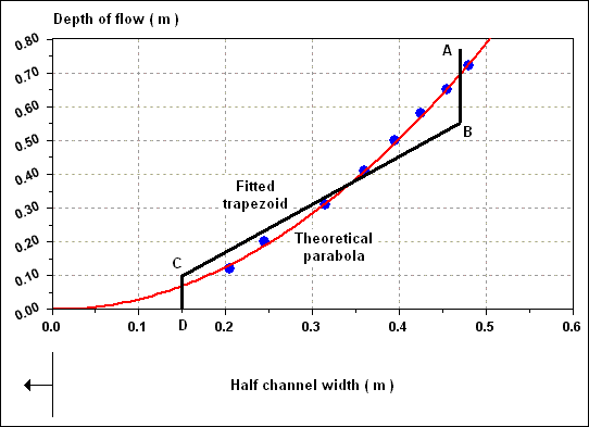
Both are satisfactorily close to the ideal value of 0.305 m / s. In practice each channel would have its own control,
however the width would be one - fifth that of the single flume. Thus ;
H = { ( Q / 5 ) / [ ( 1.71 ) ( 0.67 ) ( W / 5 ) ] } 3 / 2
is unchanged.
Scouring Velocities...
In practice grit channels operate by using the different scouring rates of grit and the lighter organic materials.
It is sometimes useful to calculate the velocity at which different materials will remain suspension, once particles
have been deposited, the system becomes extremely complex. The scouring of grit may be described by the Shields
formula ;
V = [ ( 8 K / f ) ( g ) ( R D - 1 ) ( d ) ] 1 / 2
where ; V : velocity at which the particle will begin to scour ( m / s ), K : a constant ( which varies with Reynolds
number ) between 0.03 to 0.06, f : friction factor ( 0.03 is a common value ), g : gravitational acceleration ( m /
s 2 ), R D : specific gravity of the particle and d : particle diameter.
Example 2-7 :
Assuming a mean velocity of 0.305 m / s determine the size of spherical grit particle ( R D = 2.65 ) and
spherical organic material ( R D = 1.05 ) which will remain in suspension in a grit channel for which
K = 0.05 and f = 0.03.
Calculation :
d = [ ( V 2 ) ( f ) ] / [ ( 8 ) ( K ) ( g ) ( R D - 1 ) ]
For grit ;
d = [ ( 0.305 2 ) ( 0.03 ) ] / [ ( 8 ) ( 0.05 ) ( 9.81 ) ( 1.65 ) ] = 0.43 x 10 - 3 m
For the organics ;
d = [ ( 0.305 2 ) ( 0.03 ) ] / [ ( 8 ) ( 0.05 ) ( 9.81 ) ( 0.05 ) ] = 14 x 10 - 3 m