|
Oracle® Business Intelligence Discoverer Plus User's Guide
10g Release 2 (10.1.2.1) B13915-04 |
|
 Previous |
 Next |
|
Oracle® Business Intelligence Discoverer Plus User's Guide
10g Release 2 (10.1.2.1) B13915-04 |
|
 Previous |
 Next |
This chapter explains how to use Discoverer Plus Relational's totals to answer typical business questions. For example, what is the total sales figure for January? This section contains the following topics:
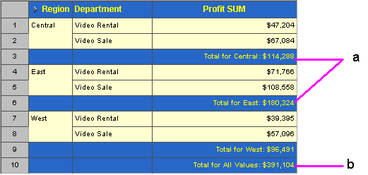
Totals are worksheet items that enable you to quickly and easily summarize rows and columns. For example, to calculate the sum of a column of profit figures, or to calculate the average of a row of sales figures. You can then use the totals to analyze the worksheet data.
Figure 14-1 A Discoverer worksheet with totals
You use Discoverer totals to calculate:
the result of applying a calculation to totals (the SUM - for more information, see "When to use SUM instead of Cell SUM")
the result of adding values (the Cell SUM - for more information, see "When to use Cell SUM instead of SUM")
the number of values (the Count)
the lowest of the values (the Minimum)
the highest of the values (the Maximum)
the square root of the variance (the Standard Deviation)
the amount of variance in a set of values (the Variance)
When a worksheet contains totals, you can:
display the totals (or turn the totals on)
hide the totals (or turn the totals off)
When creating totals, note that table worksheets and crosstab worksheets have the following differences:
On table worksheets you apply grand totals to columns. Here, you position totals at the bottom of a column.
On crosstab worksheets you can apply grand totals to either columns or rows. Here, you position totals either at the bottom of a column or on the right hand side of a row.
When you create totals in Discoverer, you can select one of two functions to calculate the sum of a column or row that contains a calculation:
SUM (Discoverer default) - use this to apply the calculation to the total
Cell SUM - use this to apply the calculation to individual values, then add the calculated values. In other words, you simply add up values in the column or row
You typically use SUM rather than Cell SUM when you add items containing:
analytic functions (e.g. Rank and NTILE)
aggregated (sum total) items (e.g. AVG and VARIANCE)
In this example, you use SUM to calculate an overall average sales figure per employee by region.
Figure 14-2 Using SUM to calculate the average sales per employee

In the figure above, the worksheet contains four items, including the calculation item Avg sales per emp. When you calculate the total for the Avg sales per emp item, you want to apply the calculation to the totals for the Sales SUM and No. of employees items. In other words, the intended total value for the Avg sales per emp item is 11,428 (i.e. 400,000/35).
Note: If you used Cell SUM in this example, you would sum the Avg sales per emp item column. This would result in the unintended total value 36,666 (i.e. 10,000 + 20,000 + 6,666).
You typically use Cell SUM rather than SUM when you simply want to add a row or column of values.
In this example, you use Cell SUM to calculate an overall total sales target for individual sales targets (i.e. an increase of ten units).
Figure 14-3 Using Cell SUM to calculate an increase in sales
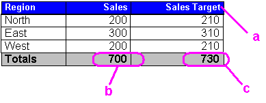
In the figure above, the worksheet contains three items, including the calculation item Sales Target. When you calculate a total for the Sales Target item, you want to sum the values in the column. In other words, the intended total value for the Sales Target item is 730 (210+310+210).
Note: If you used SUM in this example, you would apply the calculation to the total for the Sales column. This would result in the unintended total value 710 (700+10).
If you migrate workbooks containing totals from earlier versions of Discoverer to OracleBI Discoverer, you might want to:
check that the total values are consistent with how total values were calculated in the earlier version of Discoverer
where necessary, change totals in workbooks from SUM to Cell SUM or from Cell SUM to SUM
Aggregated values in Discoverer are:
values that Discoverer calculates when you add a worksheet total to a worksheet
For example, the table worksheet below contains a worksheet total (i.e. displayed as Sum: $877,594) that aggregates the Sales Sum values for regions to create a yearly total.

For more information about worksheet totals, see "What are totals?".
outline values that Discoverer calculates for you on a crosstab worksheet (if the worksheet style is set to outline)
For example, in the crosstab worksheet below Discoverer adds up the Profit Sum and Sales Sum for Chicago and Louisville to create aggregated values for the Central region (i.e. $49,246, $77,668).

Note: Discoverer calculates aggregate values on a crosstab worksheet if the worksheet uses the Outline style (i.e. if you select the Outline option in the Crosstab style drop down list on the "Options dialog: Sheet tab").
Linear calculations are worksheet calculations that Discoverer aggregates by simply adding up a series of data points. For example, in the crosstab worksheet below Discoverer adds up the Profit Sum and Sales Sum for Chicago and Louisville to create aggregated values for the Central region (i.e. $49,246, $77,668).

Non-linear calculations are worksheet calculations that Discoverer aggregates by adding up data points and applying the calculation to the result. For example, in the crosstab worksheet below Discoverer calculates the aggregated value for the Sales Margin item by applying the calculation 'Profit Sum/Sales SUM' to the aggregated values for Profit Sum and Sales Sum. In other words Discoverer calculates the aggregated value for the Sales Margin item for the Central region as 0.634 (i.e. 49,246/77,668), not as 1.322 (i.e. 0.708 + 0.614).

If a worksheet contains totals, you can display or hide the totals, as follows:
You display totals on a worksheet when you want to use them to analyze worksheet data.
You hide totals on a worksheet when you do not need to use them to analyze worksheet data.
To display or hide totals:
Display the worksheet that you want to analyze.
Choose Tools | Totals to display the "Edit Worksheet dialog: Select Items tab: Calculations tab".
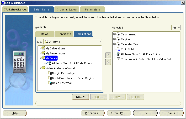
The Calculations tab lists existing calculations, percentages, and totals available in the worksheet. Active totals are marked with a tick symbol (or check mark) in the Available list and are also displayed in the Selected list.
To display an existing total, move the total from the Available list to the Selected list.
To hide an existing total, move the total from the Selected list to the Available list.
Click OK to close the Calculations tab and display the worksheet.
Discoverer refreshes the worksheet.
Notes
You can also display existing totals in the following way:
If the Available Items pane is displayed, drag and drop a total from the Calculations tab to the worksheet.
You can also hide totals in the following way:
If the Selected Items pane is displayed, right-click on a total in the Selected Items list and select Remove from Worksheet.
To remove a total from the worksheet permanently, you delete the total (for more information, see "How to delete totals").
You create totals to analyze a worksheet in a new way. For example, to calculate a sum for a list of sales figures, or to find the average of a list of profit figures.
To create a total on a table worksheet or crosstab worksheet:
Display the worksheet that you want to analyze.
Choose Tools | Totals to display the "Edit Worksheet dialog: Select Items tab: Calculations tab".

The Calculations tab lists existing calculations, percentages, and totals available in the worksheet. Active totals are marked with a tick symbol (or check mark) in the Available list and are also displayed in the Selected list.
Click New and select New Total from the drop down list to display the "New Total dialog".
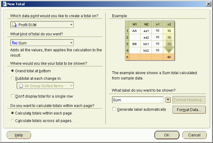
Under Which data point would you like to create a total on?, select the item that you want to summarize from the drop down list.
Note: You can also create totals for all numeric items on the worksheet by selecting All Data Points from the drop-down list.
Under What kind of total do you want?, select a total type from the drop down list.
For example, choose Sum to add the values, or choose Average to calculate a mean.
Under Where would you like your total to be shown?, choose where you want to display the total.
For example, select the Grand total at bottom radio button to calculate a grand total for a column and place it after the last row of the table.
Note: Positioning options are different depending on the type of worksheet, as follows:
on table worksheets, you can position the total at the bottom of the worksheet
on crosstab worksheets, you can position the total at the bottom of the worksheet or on the right of the worksheet
If you select the Subtotal at each change in radio button, select the item on which to group the data from the drop down list.
For example, if you sort the data by region you might want to see profits by region. If so, select region as the data item and Discoverer will display the total profit for each region on a separate line.
Under What label do you want to be shown?, do one of the following:
type in a label for the total
use the drop down list to insert variable values into the label.
Note: Select the Generate label automatically? check box if you want Discoverer to generate a label for you.
Click OK to save the details and close the dialog.
Click OK to close the Calculations tab and return to the worksheet.
Discoverer calculates the total and displays it on the worksheet.
Notes
You can also create a new total in the following ways:
Select the worksheet item for which you want to create a total, then select the New Total option on the Standard toolbar and choose one of the total types available.
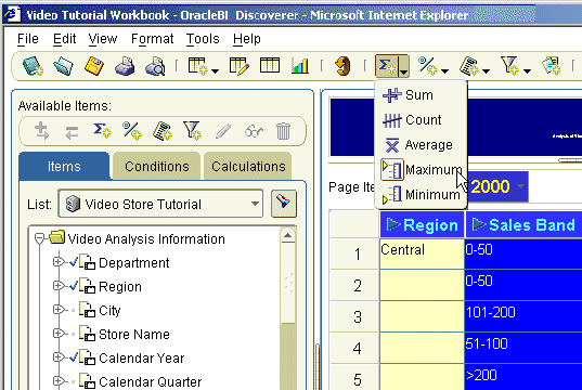
If the Available Items pane is displayed, select the New Total option on the Available Items toolbar (for more information, see "Available Items pane").
If the Available Items pane is displayed, display the Calculations tab, right-click on My Totals, and select New Total.
You edit totals when you want to change the way that they behave. For example, to change where a total is displayed on the worksheet.
To edit a total:
Display the worksheet that you want to analyze.
Choose Tools | Totals to display the "Edit Worksheet dialog: Select Items tab: Calculations tab".

The Calculations tab lists existing calculations, percentages, and totals available in the worksheet. Active totals are marked with a tick symbol (or check mark) in the Available list and are also displayed in the Selected list.
Select a total in the Available list.
Click Edit to display the "Edit Total dialog".
Edit the total details as required.
Click OK to save the details and close the Edit Total dialog.
Click OK to close the Calculations tab and return to the worksheet.
Discoverer refreshes the worksheet.
Notes
You can also edit totals in the following way:
If the Available Items pane is displayed, display the Calculations tab, right-click on a total, and select Edit.
You can change the format of totals on a worksheet using Format | Item Formats to display the "Format dialog". Then, select the total from the item list and choose Format Heading or Format Data.
You delete totals when you no longer want to use them, and want to remove them permanently from a worksheet. For example, you might have created a temporary total to produce an ad hoc report and now want to remove this total from the worksheet.
Note: If you want to remove the total from the worksheet without deleting it permanently, you can hide the total (see "How to display or hide totals").
To delete a total:
Display the worksheet that you want to analyze.
Choose Tools | Totals to display the "Edit Worksheet dialog: Select Items tab: Calculations tab".

The Calculations tab lists existing calculations, percentages, and totals available in the worksheet. Active totals are marked with a tick symbol (or check mark) in the Available list and are also displayed in the Selected list.
Select a total in the Available list.
Click Delete.
Click OK to close the Calculations tab and return to the worksheet.
Discoverer refreshes the worksheet.
Notes
You can also delete totals in the following way:
If the Available Items pane is displayed, display the Calculations tab, right-click on a total, and select Delete.
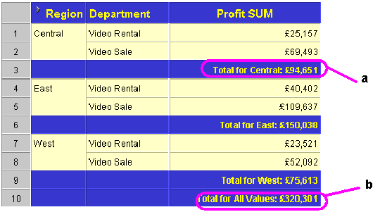
Example 1: In this example, the worksheet contains profit values for regions. You want to display a sub-total for each region, and a grand total for all regions.
Figure 14-4 Displaying a total on a table worksheet
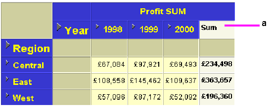
Example 2: In this example, a crosstab worksheet contains profit values for regions in different years. You want to display a profit total of all three years for each region.
Figure 14-5 Displaying a total on a crosstab worksheet
Example 3: In this example, the worksheet contains profit and sales values for each quarter in the Central region. You want to display a total profit figure and a total sales figure.
Figure 14-6 Displaying two totals on a crosstab worksheet
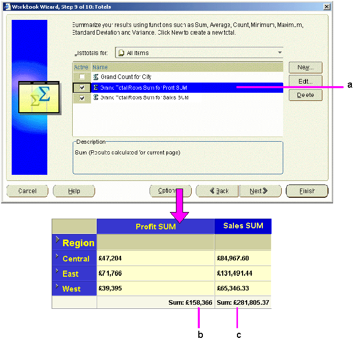
Notice that the two totals are displayed on the same row. When a crosstab has multiple totals displayed, Discoverer automatically puts them on the same row.
The following examples show how aggregation options specified on the "Worksheet Properties dialog: Aggregation tab" affect how Discoverer displays aggregated values.
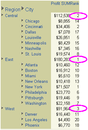
In this example (using an Oracle9i database), you want to calculate a ranked list of cities based on profits. You want the highest profits to have the highest rank. You create a Discoverer calculation called 'Rank' with the following formula:
RANK() OVER(PARTITION BY "Calendar Year" ORDER BY "Profit SUM" DESC)
You want Discoverer to calculate the 'Rank' aggregated value as follows:
rank regions against each other (e.g. the East region is ranked 1 with profits of $180,283 and the Central region is ranked 2 with profits of $112,538)
rank cities against each other (e.g. New York is ranked 1 with profits of $71,507, and Cincinnati is ranked 2 with profits of $34,406)
The worksheet below shows how Discoverer calculates the ranks if you select the Show the aggregated value computed by the database. The database uses the same aggregation method as Discoverer option on the "Worksheet Properties dialog: Aggregation tab".
The table below shows how Discoverer calculates the 'Rank' aggregated values for the different options on the "Worksheet Properties dialog: Aggregation tab".
Table 14-1 Explanation of fields
This example (using an Oracle9i database) shows how Discoverer does not aggregate repeated values, whichever aggregation option you choose on the "Worksheet Properties dialog: Aggregation tab".
In this example, a worksheet displays sales values (i.e. the Sales SUM item) for regions for each year. The worksheet also displays the target sales value set by the company (i.e. the Target Sales SUM item) for each region. Each region has the same target sales value. You create a Discoverer total to calculate total values for each year.
It is not meaningful to aggregate Target Sales Sum values at the Year level because there is no logical relationship between the Sales item and the Target Sales item. If you are familiar with entity-relationship diagrams, the figure below shows that this is because the Sales SUM item is dimensioned by store (i.e. in the Sales Facts table) but the Target Sales Sum item is dimensioned by date (i.e. in the Date table).
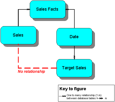
Therefore, you want Discoverer to display a non-aggregable label (e.g. N.A.) for the yearly total values for the Target Sales Sum item. The worksheet below shows how Discoverer displays a non-aggregable label (i.e. N.A.) for the yearly totals for the Target Sales Sum item (regardless of which aggregation option you choose on the "Worksheet Properties dialog: Aggregation tab".
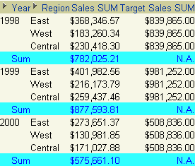
The table below shows how Discoverer the Target Sales Sum aggregates are calculated for the different radio button options on the "Worksheet Properties dialog: Aggregation tab".
Table 14-2 Explanation of fields
| Check box selected | What value is displayed? |
|---|---|
|
Show the aggregated value calculated by the database. The database uses the same aggregation method as Discoverer |
N.A. |
|
Show <Non-aggregable label>, the "values that cannot be aggregated" option, set on the Sheet Format tab |
N.A. |
|
Show the sum of the values displayed in the contributing cells |
N.A. |