|
Oracle® Business Intelligence Discoverer Plus User's Guide
10g Release 2 (10.1.2.1) B13915-04 |
|
 Previous |
 Next |
|
Oracle® Business Intelligence Discoverer Plus User's Guide
10g Release 2 (10.1.2.1) B13915-04 |
|
 Previous |
 Next |
This appendix contains the following sections:
"How to find more information about Oracle analytic functions"
"About using parameters to provide dynamic input to calculations"
For more information about Oracle functions in general, refer to the following Oracle publications:
Oracle SQL Reference
Oracle Data Warehousing Guide
The examples in the following sections use the Video Stores Tutorial supplied with Discoverer. If you do not have the Video Stores Tutorial installed, contact the Discoverer manager.
Note: If that database version that you are using does not support IF or CASE statements, you can use DECODE instead. Alternatively, you can create a PL/SQL function in the database.
For more information about how to create calculations, see "How to create calculations".
You often use parameters to provide dynamic input to calculations. This enables other values to be entered arbitrarily for more effective analysis. In other words, to provide a different value to a calculation, you simply refresh the worksheet and enter a new value in the "Edit Parameter Values dialog".
Parameter values used in calculations are prefixed with a colon (:). For example, a parameter called Hypothetical Value would be referenced in a calculation as follows:
RANK(:Hypothetical Value) WITHIN GROUP(ORDER BY Profit DESC NULLS FIRST)
For more information about using parameter values in calculations, see "About using parameters to collect dynamic user input".
The examples in this section show you how to use basic functions with Discoverer to manipulate and analyze data.
Examples:
Notes
Examples in this section use a selection of commonly used commands. For a complete list of commands and their full syntax, refer to the Oracle SQL and warehousing guides.
For more information on how to create calculations, see "Using calculations".
Example: Calculate the number of rows returned by a query
This example calculates the number of rows returned by a query using the Oracle function ROWCOUNT().
| Worksheet options | Set to: |
|---|---|
| Items | Video Analysis Information: Calendar Year, Region, City, Sales SUM |
| Sort Order | Year, Region, City |
| Conditions | Department = Video Sale OR Department = Video Rental
Calendar Year = 2000 Region = Central |
| Calculation Name | Rows returned |
| Calculation | ROWCOUNT |
Figure A-1 Worksheet containing the Rows returned calculation
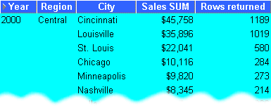
The worksheet shows the number of rows returned for each city in the central region for the year 2000.
Notes
ROWCOUNT does not count NULL values. To calculate the number of rows returned by a query, including NULL values, do the following:
first create a temporary item called 'One record', with the formula = '1'
create a calculation called 'Rows returned' to count the occurrences of One record, with the formula = SUM(Video Sales Analysis.One record)
Example: Calculate a 25% increase in sales
This example calculates a 25% increase in sales.
| Worksheet options | Set to: |
|---|---|
| Items | Video Analysis Information: Calendar Year, Region, City, Sales SUM |
| Sort Order | Year, Region, City |
| Conditions | Department = Video Sale OR Department = Video Rental
Calendar Year = 2000 Region = Central |
| Calculation Name | 25% Increase |
| Calculation | Sales SUM * 1.25 |
Figure A-2 Worksheet containing the 25% sales increase calculation.
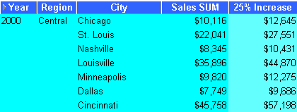
The worksheet shows a 25% increase in sales for cities in the central region.
Example: Convert text to upper-case
As well as the extensive range of mathematical functions available in Discoverer, you also have access to a wide range of number and text formatting functions. This example uses a calculation to re-format City text data to upper-case
| Worksheet options | Set to: |
|---|---|
| Items | Video Analysis Information: Calendar Year, Region, City, Sales SUM |
| Sort Order | Year, Region |
| Conditions | Department = Video Sale OR Department = Video Rental
Calendar Year = 2000 Region = Central |
| Calculation Name | City(Upper Case) |
| Calculation | UPPER(City) |
Figure A-3 Worksheet containing the City(Upper Case) calculation
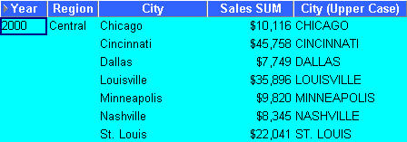
The figure above shows a worksheet containing the city names for the central region converted to upper case.
The examples in this section show you how to use the Oracle analytic functions with Discoverer to perform detailed data analysis.
This section contains the following topics:
"About analytic functions and drilling into and out of data"
"About differences between PERCENTILE_CONT and PERCENTILE_DISC"
Notes
Examples in this section use a selection of commonly used commands. For a complete list of commands and their full syntax, refer to the Oracle SQL Reference and the Oracle Data Warehousing Guide.
For more information on how to create calculations, see "Using calculations".
Hint: You can also use analytic function templates to quickly and easily create calculations based on the most popular analytic functions (for more information, see "How to create a new calculation using an analytic function template".
Analytic functions are classified in the following categories:
Ranking - Address business questions like: 'What are the top 10 and bottom 10 salespeople per region?'.
Banding - Address business questions like 'What brands make up 25% of sales?'.
Windowing - Address business questions like 'What is the 13-week moving average of a stock price?' or 'What is the cumulative sum of sales per region?'.
Reporting Aggregates - After a query has been processed, aggregate values like the number of resulting rows, or the sum of a column in a set of rows. Address questions like 'What are each product's Sales as a percentage of Sales for its product group?'.
Lag/Lead - Address business questions like 'What was the value of sales for the same period one year ago?'.
Statistics - Perform statistical analysis with Business Intelligence OLAP/spreadsheet applications. For example, covariance and linear regression functions.
When you use analytic functions, note that they have a precise definition which might not change as you drill, pivot, or sort the result set. For example, if you use the Rank function to assign ranks to sales figures partitioned by quarter, if you drill down to the month level, the rank still only applies to the quarter level.
Discoverer Plus Relational provides easy-to-use templates for the most popular analytic functions (for more information, see "What analytic function templates are available in Discoverer?").
If you want to create an analytic function that does not have a template, you can either type or paste it directly into the Calculation field on the "New Calculation dialog", or you can select it from the function list.
If you select analytic functions from the function list on the "New Calculation dialog", Discoverer copies a blank analytic function into the Calculation field. The blank analytic function contains expr prompts for missing values that tell you what information you might need to provide. The expr prompts are designed to cover most types of usage, and should be used only as a guide. In other words, you will not always need to use every expr prompt to define an analytic function.
For example, when you select the RANK analytic function in the "New Calculation dialog", Discoverer types the following text into the Calculation field:
RANK() OVER (PARTITION BY expr1 ORDER BY expr2)
Although you can define a complex function using both expressions (expr1 and expr2), you can often define a simple function using only the ORDER BY expression; for example:
RANK() OVER(ORDER BY 'Sales')
This example ranks sales figures (defined in the 'Sales' item).
Notes
By default, results data is sorted in ascending order (ASC), nulls first (NULLS FIRST).
For more information about entering analytic functions, see "More about analytic functions expressions".
This section contains examples of rank functions.
Ranking functions compute the ranked list position of an item with respect to other items in an ordered list.
Examples:
Hint: You can also use analytic function templates to quickly and easily create calculations based on ranking functions (for more information, see "How to create a new calculation using an analytic function template".
This example calculates the ranked list position of a set of sales figures.
| Worksheet options | Set to: |
|---|---|
| Items | Video Analysis Information: Calendar Year, Region, City, Sales SUM |
| Sort Order | Rank Sales, Year, Region |
| Conditions | Department = Video Sale OR Department = Video Rental
Calendar Year = 2000 |
| Calculation Name | Rank Sales |
| Calculation | RANK() OVER(ORDER BY Sales SUM DESC) |
Figure A-4 Worksheet containing the Rank Sales calculation
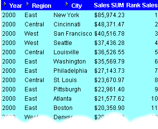
The worksheet shows the ranked list position of sales figures for cities in the year 2000.
Notes
By default, ranked results data is sorted in ascending order (ASC), nulls first (NULLS FIRST). The additional DESC parameter sorts the results in descending order, which ranks the highest value with the Rank 1.
This example calculates the ranked list position of a set of sales figures within each region.
| Worksheet options | Set to: |
|---|---|
| Items | Video Analysis Information: Calendar Year, Region, City, Sales SUM |
| Sort Order | Year, Region |
| Conditions | Department = Video Sale OR Department = Video Rental
Calendar Year = 2000 |
| Calculation Name | Rank sales within Region |
| Calculation | RANK() OVER(PARTITION BY Year, Region ORDER BY Sales SUM DESC) |
Figure A-5 Worksheet containing the Rank sales within Region calculation
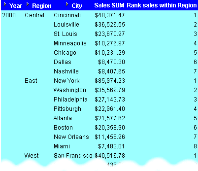
The worksheet shows the ranked list position of sales figures for cities grouped by region within year.
Notes
By default, ranked results data is sorted in ascending order (ASC), nulls first (NULLS FIRST). The additional DESC parameter sorts the results in descending order, which ranks the highest value with the Rank 1.
This example calculates the ranked list position of a set of sales figures and displays the top three selling cities.
| Worksheet options | Set to: |
|---|---|
| Items | Video Analysis Information: Calendar Year, Region, City, Sales SUM |
| Sort Order | Year, Region |
| Conditions | Department = Video Sale OR Department = Video Rental
Calendar Year = 2000 Rank Top <= 3 |
| Calculation Name | Rank Top |
| Calculation | RANK() OVER(PARTITION BY Year, Region ORDER BY Sales SUM DESC) |
Figure A-6 Worksheet containing the Rank Top calculation used in a condition
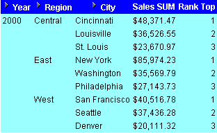
The worksheet shows a ranked list of the top three highest sales figures for each region within year.
Notes
By default, ranked results data is sorted in ascending order (ASC), nulls first (NULLS FIRST). The additional DESC parameter sorts the results in descending order, which ranks the highest value with the Rank 1.
Hint: To quickly filter the list to the first, second, or third ranked cities, pivot the Rank Top item to the page axis.
This example calculates the ranked list position of a set of sales figures and displays the top three and bottom three performing cities per region.
| Worksheet options | Set to: |
|---|---|
| Items | Video Analysis Information: Calendar Year, Region, City, Sales SUM |
| Sort Order | Year, Region, Rank Top |
| Conditions | Department = Video Sale OR Department = Video Rental
Calendar Year = 2000 Rank Top <= 3 OR Rank Bottom <= 3 |
| Calculation Name | Rank Top |
| Calculation | RANK() OVER(PARTITION BY Year, Region ORDER BY Sales SUM DESC) |
| Additional Calculations Required | Rank Bottom = RANK() OVER(PARTITION BY Year, Region ORDER BY Sales SUM ASC) |
Figure A-7 Worksheet containing the Rank Top calculation used in a condition
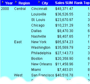
The worksheet shows a ranked list of the three highest and three lowest sales figures for each region within year.
Notes
This analysis involves three steps:
Assign ranks to Cities on Sales SUM in descending order, as Rank Top.
Assign ranks to Cities on Sales SUM in ascending order, as Rank Bottom.
Displaying only Rank Top, filter the data using a Condition to return only the top three and bottom three ranked Cities.
In the example, in the 'Central' Region, the top three cities are ranked 1, 2, and 3; the bottom three cities are ranked 5, 6, and 7. In the 'East' Region, the top three cities are ranked 1, 2, and 3; the bottom three cities are ranked 6, 7, and 8, and so on.
This section contains examples of banding functions.
Banding is a type of ranking that divides a list of values in a partition into a specified number of groups called bands (also known as buckets) and assigns each value to a band.
Examples:
Hint: You can also use analytic function templates to quickly and easily create calculations based on banding functions (for more information, see "How to create a new calculation using an analytic function template".
Two common types of banding are:
Banding by value - this divides values into groups according to their value (also known as equi-width bands). This type of analysis is also known as frequency distribution.
Here, the function typically takes the largest value minus the lowest value, and divides the result by the number of bands required. This value defines the range of each Band.
Values are then assigned to bands according to which range they fall into. Therefore, the number of values in each Band might differ. For example, if we have 100 values and divide them into four equi-width bands, each band might contain different numbers of values.
Use the GREATEST function or the CASE function to produce equi-width bands based on value.
Note: If that database version that you are using does not support IF or CASE statements, you can use DECODE instead. Alternatively, you can create a PL/SQL function in the database.
Hint: You can also use the WIDTH_BUCKET function to produce equi-width bands (see "Example: Producing equi-width bands using WIDTH_BUCKET").
Banding by rank - this divides values into groups according to their rank (also known as equi-height bands). This type of analysis is also known as percentile analysis (e.g. 4 bands give quartiles).
Here, the function divides the number of values in the partition by the number of bands, which gives the number of values in each band. An equal number of values are then placed in each band. For example, if we have 100 values and divide them into four equi-height bands, each band contains 25 values.
Use the NTILE function to produce equi-height bands based on rank.
This example divides sales figures into bands according to their value (e.g. for frequency analysis). For more information, see "Example: Banding by value (2)".
| Worksheet options | Set to: |
|---|---|
| Items | Video Analysis Information: Calendar Year, Region, City, Sales SUM |
| Sort Order | Year, Region |
| Conditions | Department = Video Sale OR Department = Video Rental
Calendar Year = 2000 Region = Central |
| Calculation Name | Sales Bands |
| Calculation | GREATEST(1,4-FLOOR((Sales SUM-Min Sales for Region)/GREATEST(1,FLOOR((Max Sales for Region-Min Sales for Region+1)/4)))) |
| Additional Calculations Required | Max Sales for Region = MAX(Sales SUM) OVER(PARTITION BY Region,Year)
Min Sales for Region = MIN(Sales SUM) OVER(PARTITION BY Region,Year) |
Figure A-10 Worksheet containing the Sales Bands calculation
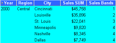
The worksheet shows equi-width bands for sales figures for cities in the central region within year.
Notes
Using the Central Region and Year 2000 as an example, this function takes the largest value (45,758) minus the smallest value (7,749) and divides it by four ((45,758-7,749)/4), giving four equal Bands of 9,502.25. This gives four bands with the following ranges:
Band 1 - 36,255.75 to 45,758
Band 2 - 26,753.5 to 36,255.75
Band 3 - 17,251.25 to 26,753.5
Band 4 - 7,749 to 17,251.25
Each value is placed in one of the four Bands depending on which range the Sales SUM value falls into.
The FLOOR function returns the largest integer equal to or less than n. For example, in Dallas, the expression FLOOR(Sales SUM-Min Sales for Region) returns the smallest integer value from 7,749 minus 7,749, which returns 0. When used in conjunction with the GREATEST function (see calculation above), the expression GREATEST(1,4-FLOOR((Sales SUM-Min Sales for Region) returns the largest value from either 1 or, 4 minus the smallest integer value from 7,749 minus 7,749 (4 minus 0 equals 4). In other words, the expression returns the value 4.
You can also use the WIDTH_BUCKET function to produce equi-width bands (see "Example: Producing equi-width bands using WIDTH_BUCKET").
This example divides sales figures into bands according to their value. The example creates the same results as the example in "Example: Banding by value (1)", except that it uses a CASE statement rather than the GREATEST function (e.g. for frequency analysis).
| Worksheet options | Set to: |
|---|---|
| Items | Video Analysis Information: Calendar Year, Region, City, Sales SUM |
| Sort Order | Year, Region |
| Conditions | Department = Video Sale OR Department = Video Rental
Calendar Year = 2000 Region = Central |
| Calculation Name | Sales Bands 2 |
| Calculation | CASE WHEN Sales SUM < Q1 THEN 4 WHEN Sales SUM < Q2 THEN 3 WHEN Sales SUM < Q3 THEN 2 WHEN Sales SUM >= Q3 THEN 1 END |
| Additional Calculations Required | MAX Sales = MAX(Sales SUM) OVER(PARTITION BY Year)
MIN Sales = MIN(Sales SUM) OVER(PARTITION BY Year) Range = (MAX Sales - MIN Sales)/4 Q1 = MIN Sales + Range Q2 = MIN Sales + (Range*2) Q3 = MAX Sales - Range |
Figure A-11 Worksheet containing the Sales Bands 2 calculation
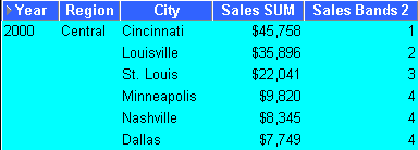
The worksheet shows equi-width bands for sales figures for cities in the central region within year.
Notes
This function uses a series of IF statements in the form of a CASE function to assign sales figures into bands (see Band ranges below).
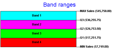
You can also use the WIDTH_BUCKET function to produce equi-width bands (see "Example: Producing equi-width bands using WIDTH_BUCKET").
This example divides sales figures into two bands according to their rank (e.g. for percentile analysis).
| Worksheet options | Set to: |
|---|---|
| Items | Video Analysis Information: Calendar Year, Region, City, Sales SUM |
| Sort Order | Year, Region |
| Conditions | Department = Video Sale OR Department = Video Rental
Calendar Year = 2000 Region = Central |
| Calculation Name | Sales Bands 3 |
| Calculation | NTILE(2) OVER(PARTITION BY Year, Region ORDER BY Sales SUM DESC) |
Figure A-12 Worksheet containing the Sales Bands 3 calculation
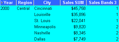
The worksheet shows equi-height bands for sales figures for cities in the central region within year.
Notes
Using the Central Region and Year 2000 as an example, this function takes the number of values (which is six) and divides it by two, giving three values per Band. It then takes the list of values ordered by Sales SUM and places values one, two, and three in band 1, values four, five, and six in band 2.
This section contains examples of windowing functions.
Windowing functions are used to compute aggregates using values from other rows. For example, cumulative, moving, and centered aggregates.
Note: For more information about using row-based and time-based intervals, see "Examples of using row-based and time-based intervals".
Examples:
Hint: You can also use analytic function templates to quickly and easily create calculations based on windowing functions (for more information, see "How to create a new calculation using an analytic function template".
Two common types of windowing are:
Windowing with time-based intervals - here, a time-based interval is based on a value relative to an existing value. For example, three months preceding a date value.
Note: Time-based intervals are also known as logical offsets.
Time-based intervals are useful when data has missing rows. For example, you might not have seven rows for sales figures for seven days in a week, but you still want to find a weekly average.
For example, if we have a list of monthly sales figures, a logical window might compute a moving average of the previous three months (inclusive of the current month). When calculating the average, the calculation assumes a NULL value for months missing from the list. In the example below, the three-month moving average for November assumes NULL values for the missing months September and October.
Windowing with row-based intervals - here, a row-based interval is based on a value that is a specified number of rows from an existing value. For example, three rows from the current item.
Note: Row-based intervals are also known as physical offsets.
Row-based intervals are useful when data does not have missing rows. For example, if you know that you have seven rows for sales figures for seven days in a week, you can calculate a weekly average by starting the interval six rows before the current row (inclusive).
For example, if we have a list of monthly sales figures, a physical window might compute a moving average of the previous three rows. When calculating the average, the calculation ignores months missing from the list. In the example below, the three-month moving average for November uses June, July, and November in the calculation.
Note: For more information about using row-based and time-based intervals, see "Examples of using row-based and time-based intervals".
This example uses a time-based interval to calculate a moving three month sales average.
Note: Moving averages are also known as rolling averages.
| Worksheet options | Set to: |
|---|---|
| Items | Video Analysis Information: Calendar Year, Calendar Month, Sales SUM |
| Sort Order | Year, Month |
| Conditions | Department = Video Sale OR Department = Video Rental
Calendar Year = 2000 Region = Central |
| Calculation Name | Moving Average |
| Calculation | AVG(Sales SUM) OVER(ORDER BY "Calendar Month" RANGE INTERVAL '2' MONTH PRECEDING) |
Figure A-15 Worksheet containing the Moving Average calculation
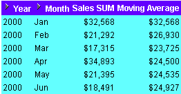
The worksheet shows a moving three month average for sales figures for months in the year 2000.
Notes
Note that you define the RANGE INTERVAL as '2', not '3', even though you want a three month window. This is because the window expression implicitly includes the current row. Therefore, in this example, the INTERVAL '2' plus the current row gives a total of three months (2 + current row = 3).
This example uses a row-based interval to calculate the cumulative value of sales.
| Worksheet options | Set to: |
|---|---|
| Items | Video Analysis Information: Calendar Year, Region, City, Sales SUM |
| Sort Order | Year, Region |
| Conditions | Department = Video Sale OR Department = Video Rental
Calendar Year = 2000 Region = Central |
| Calculation Name | Cumulative Total |
| Calculation | SUM(Sales SUM) OVER(PARTITION BY "Calendar Year", Region ORDER BY Sales SUM ROWS UNBOUNDED PRECEDING) |
Figure A-16 Worksheet containing the Cumulative Total calculation
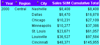
The worksheet shows a cumulative total for sales figures for cities in the central region.
This example uses a time-based interval to calculate sales figures for previous years. This enables you to compare sales figures over different years, or compare previous years' sales figures with other values, such as spending in previous years.
| Worksheet options | Set to: |
|---|---|
| Items | Video Analysis Information: Calendar Year, Sales SUM |
| Sort Order | N/A |
| Conditions | N/A |
| Calculation Name | Sales Last Year |
| Calculation | SUM(Sales SUM) OVER(ORDER BY "Calendar Year" RANGE BETWEEN INTERVAL '1' YEAR PRECEDING AND INTERVAL '1' YEAR PRECEDING) |
Figure A-17 Worksheet containing the Sales Last Year calculation

For each row, the worksheet shows the sales total for the previous year.
Notes
In the example above, the Sales Last Year value for 1998 is NULL because the database does not contain information for 1997.
You can also use LAG/LEAD functions to compare values across time (see "LAG/LEAD function examples".
This section contains examples of reporting functions.
Reporting functions are used to compute aggregates.
Examples:
Hint: You can also use analytic function templates to quickly and easily create calculations based on reporting functions (for more information, see "How to create a new calculation using an analytic function template".
This example calculates annual sales.
| Worksheet options | Set to: |
|---|---|
| Items | Video Analysis Information: Calendar Year, Region, City, Sales SUM |
| Sort Order | Year, Region |
| Conditions | Department = Video Sale OR Department = Video Rental
Calendar Year = 2000 |
| Calculation Name | Annual Sales |
| Calculation | SUM(Sales SUM) OVER() |
Figure A-18 Worksheet containing the Annual Sales calculation
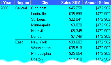
The worksheet shows the annual sales value for cities in the year 2000.
Notes
On table worksheets, the calculation displays the returned value for each row in the worksheet. To return a single value, move the calculation into the Page Items area (for more details see Additional Notes in "Example: Find the largest sales transactions in area with most sales trans'".
This example calculates the total annual sales by region.
| Worksheet options | Set to: |
|---|---|
| Items | Video Analysis Information: Calendar Year, Region, City, Sales SUM |
| Sort Order | Year, Region |
| Conditions | Department = Video Sale OR Department = Video Rental
Calendar Year = 2000 |
| Calculation Name | Annual Sales by Region |
| Calculation | SUM(Sales SUM) OVER(PARTITION BY Year, Region ORDER BY Year, Region) |
.
Figure A-19 Worksheet containing the Annual Sales by Region calculation
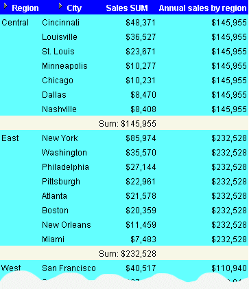
The worksheet shows the annual sales total for cities, grouped by region within year.
This example calculates the percentage of annual sales per region for each city in each year.
| Worksheet options | Set to: |
|---|---|
| Items | Video Analysis Information: Calendar Year, Region, City, Sales SUM |
| Sort Order | Year, Region, % of Annual Sales |
| Conditions | Department = Video Sale OR Department = Video Rental
Calendar Year = 2000 |
| Calculation Name | % of Annual Sales |
| Calculation | Sales SUM*100/Annual Sales by Region |
| Additional Calculations Required | Annual Sales by Region = SUM(Sales SUM) OVER(PARTITION BY Year, Region ORDER BY Year, Region) |
Figure A-20 Worksheet containing the % of Annual Sales calculation
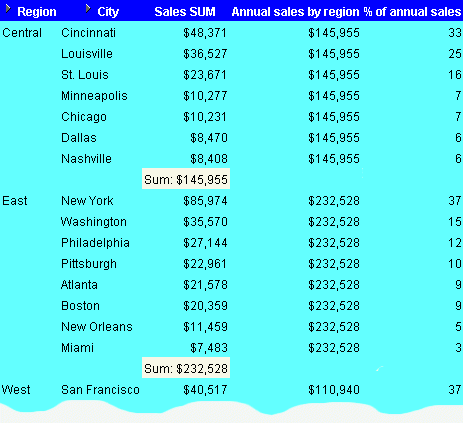
The worksheet shows sales as a percentage of annual sales, grouped by region within year.
This example calculates city sales as a percentage of total sales.
| Worksheet options | Set to: |
|---|---|
| Items | Video Analysis Information: Calendar Year, Region, City, Sales SUM |
| Sort Order | Year, Region, % of Annual Sales |
| Conditions | Department = Video Sale OR Department = Video Rental
Calendar Year = 2000 Region = Central |
| Calculation Name | % of total Sales |
| Calculation | RATIO_TO_REPORT(Sales SUM) OVER()*100 |
Figure A-21 Worksheet containing the % of Annual Sales calculation
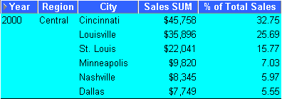
The worksheet shows the sales value for cities as a percentage of total sales.
Notes
The function RATIO_TO_REPORT computes the ratio of a value to the sum of a set of values.
This section contains examples of LAG and LEAD functions.
LAG and LEAD functions are typically used to compare values in different time periods. For example, compare sales figures in 2000 with sales figures in 2001.
LAG - provides access to more than one row of a table at the same time without a self-join.
LEAD - provides access to a row at a given offset after the current position.
You can also use windowing functions to compare values over time (see "Example: Compare sales figures across time using windowing".
Hint: You can also use analytic function templates to quickly and easily create calculations based on LAG/LEAD functions (for more information, see "How to create a new calculation using an analytic function template".
Examples:
In this example, you want to compare monthly sales figures with sales figures for the same month in the previous year. For example, to look at how January 1999 sales compare with January 1998 sales.
| Worksheet options | Set to: |
|---|---|
| Items | Video Analysis Information: Calendar Year, Calendar Quarter, Calendar Month, Sales SUM |
| Sort Order | Calendar Year, Calendar Quarter, Calendar Month |
| Conditions | Department = Video Sale OR Department = Video Rental
|
| Calculation Name | Previous Year |
| Calculation | LAG(Sales SUM,1) OVER(PARTITION BY "Calendar Month" ORDER BY "Calendar Year") |
Figure A-22 Worksheet containing the Previous Year calculation partitioned by Calendar Month
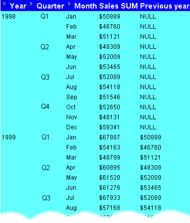
The worksheet shows contains the calculation Previous Year, which shows for each Sales SUM amount the sales amount for one year previously. For example, the Previous Year value for January 1999 is $50889, which is the Sales SUM value for January 1998.
Notes
Because there are no comparative figures for 1998, the Previous Year values for 1998 are blank.
Notice that the value '1' in the LAG(Sales SUM,1) clause calculates the value from one year previously. For example, if you changed this value to '2', you would calculate the value from two years previously.
Notice that the calculation includes the clause 'PARTITION BY Calendar Month', which gives you a value for each combination of Calendar Year (in the ORDER BY clause) and Calendar Month (in the PARTITION BY clause). In other words, the Previous Year value for February 1999 is the Sales SUM value for February 1998. If you removed this clause, you would calculate the value for the previous month (see example below). In other words, the Previous Year value for February 1999 would be the Sales SUM value for January 1999.
Figure A-23 Worksheet containing the Previous Year calculation with the partition removed
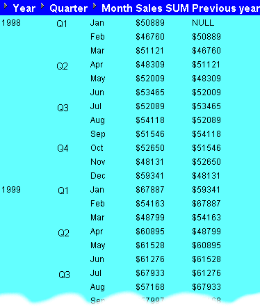
In this example, you want to calculate the percentage growth of sales across years by comparing the sales figures with sales figures for the same month in the previous year. You will do this using the comparative sales figures from example "Example: Compare sales figures across time using LAG/LEAD".
| Worksheet option | Set to: |
|---|---|
| Items | Video Analysis Information: Calendar Year, Calendar Quarter, Calendar Month, Sales SUM |
| Sort Order | Calendar Year, Calendar Quarter, Calendar Month |
| Conditions | Department = Video Sale OR Department = Video Rental
|
| Calculation Name | Growth % |
| Calculation | (Sales SUM-"Previous year")*100/"Previous year" |
| Additional Calculations Required | LAG(Sales SUM,1) OVER(PARTITION BY "Calendar Month" ORDER BY "Calendar Year") |
Figure A-24 Worksheet containing the Growth calculation
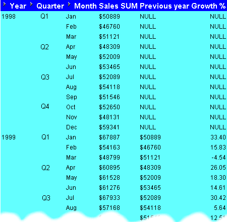
The worksheet shows contains the calculation Growth %, which shows for each month the percentage increase in sales since the previous year. For example, the Growth % value for January 1999 is 30.40% (i.e. from $50889 to $67887).
Notes
Because there are no comparative figures for 1998, the Growth values for 1998 are blank.
The calculation subtracts the Previous Year value from the Sales SUM value, then multiplies the result by the Sales SUM value divided by the Previous Year value. For example, if sales have risen from 75 to 100, the calculation becomes 25 * 1.33, giving 33.33% increase.
For more information about the calculation Previous Year, see "Example: Compare sales figures across time using LAG/LEAD".
In this example, you want to create a ranked list of sales growth, to show which months show the highest year on year increase in sales.
You will do this using the comparative sales figures and growth figures from examples "Example: Compare sales figures across time using LAG/LEAD" and "Example: Calculate sales growth across time", and a RANK function.
| Worksheet options | Set to: |
|---|---|
| Items | Video Analysis Information: Calendar Year, Calendar Quarter, Calendar Month, Sales SUM |
| Sort Order | Calendar Year, Calendar Quarter, Calendar Month |
| Conditions | Department = Video Sale OR Department = Video Rental
|
| Calculation Name | Rank Growth |
| Calculation | RANK() OVER(PARTITION BY "Calendar Year" ORDER BY "Growth %" DESC) |
| Additional Calculations Required | Previous Year = LAG(Sales SUM,1) OVER(PARTITION BY "Calendar Month" ORDER BY "Calendar Year")
Growth % = (Sales SUM-"Previous year")*100/"Previous year" |
Figure A-25 Worksheet containing the Rank Growth calculation
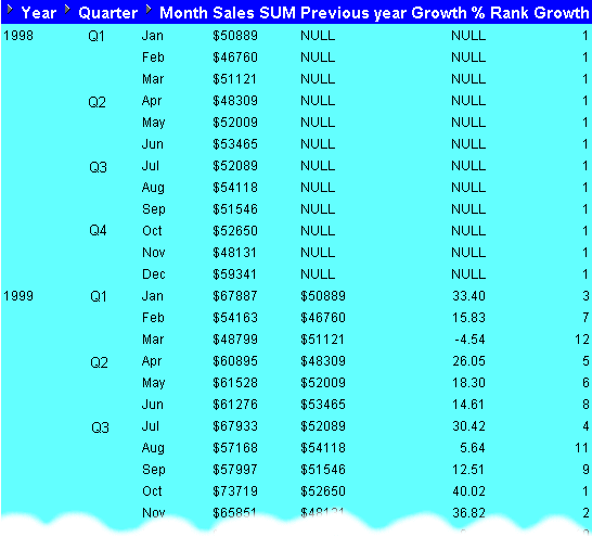
The worksheet shows the ranked list position of sales growth. For example, the Rank Growth value for January 1999 is 3, which means that January was the third best performing month (i.e. the sales growth for the month of January between 1998 and 1999 was the third highest in the ranked list).
Notes
Because there are no comparative figures for 1998, the Rank Growth values for 1998 are 1.
Looking at the example above, you can see that sales growth was highest between October 1998 and October 1999 (40.02%)
For more information about the calculation Previous Year, see "Example: Compare sales figures across time using LAG/LEAD".
For more information about the calculation Growth, see "Example: Calculate sales growth across time".
This section contains examples of statistical functions.
Statistics functions are used to compute covariance, correlation, and linear regression statistics. Each function operates on an unordered set. They also can be used as windowing and reporting functions.
Examples:
This example computes an ordinary least-squares regression line that expresses the Profit SUM per month as a linear function of its Sales SUM. The following functions are used:
SLOPE - slope of determination of the regression line
INTERCEPT - intercept of determination of the regression line
REGR_R2 - coefficient of determination of the regression line
REGR_COUNT - number of items
REGR_AVGX - average sales
REGR_AVGY - average profit
| Worksheet options | Set to: |
|---|---|
| Items | Video Analysis Information: Calendar Year, Calendar Month, Sales SUM, Profit SUM |
| Sort Order | Calendar Year |
| Conditions | Department = Video Sale OR Department = Video Rental
Calendar Year = 2000 |
| Calculations | Slope = REGR_SLOPE(Profit SUM,Sales SUM) OVER(PARTITION BY Calendar Year ORDER BY Profit SUM)
Intercept = REGR_INTERCEPT(Profit SUM,Sales SUM) OVER(PARTITION BY Calendar Year ORDER BY Profit SUM) Coefficient = REGR_R2(Profit SUM,Sales SUM) OVER(PARTITION BY Calendar Year ORDER BY Profit SUM) Count = REGR_COUNT(Profit SUM,Sales SUM) OVER(PARTITION BY Calendar Year ORDER BY Profit SUM) Average = REGR_AVGX(Profit SUM,Sales SUM) OVER(PARTITION BY Calendar Year ORDER BY Profit SUM) Average 2 = REGR_AVGY(Profit SUM,Sales SUM) OVER(PARTITION BY Calendar Year ORDER BY Profit SUM) |
Figure A-26 Worksheet containing the statistical calculations

The worksheet shows for each month the slope, intercept, coefficient, count, and average values.
Notes
For more information about regression analysis, refer to Oracle SQL Reference and Oracle Data Warehousing Guide.
When you select an analytic function in the "New Calculation dialog", Discoverer types generic text into the Calculation field to help you define the function. This generic text includes:
OVER (PARTITION BY expr1 ORDER BY expr2)
The expressions are used as follows.
OVER - indicates that the function operates on a query result set, after the other query clauses have been applied (e.g. FROM, WHERE, HAVING).
PARTITION BY - partition (or group) the query results set (e.g. PARTITION BY 'Region').
ORDER BY - specify how the results set is logically ordered (e.g. ORDER BY 'Sales SUM').
For more information about Oracle expressions, see "How to find more information about Oracle analytic functions".
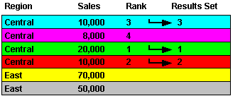
When you use analytic functions in conditions, the way that you combine them with non-analytic functions affects the Discoverer data returned by the query. The following sequencing rules apply (for more information, see "Examples of sequencing"):
Where conditions contain only non-analytic functions, these are applied before conditions that contain analytic functions. In the example below, the 'Region = 'Central' condition is applied first, then the rank is computed, then the 'Rank <= 3' condition is applied (which contains an analytic function).

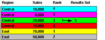
Where conditions contain a combination of non-analytic functions and analytic functions, the analytic functions are applied before the non-analytic functions. In the example below, the rank is evaluated, then the 'Rank <= 3' condition is applied, then the 'Region = 'Central' condition is applied.

To illustrate how sequencing affects the Discoverer data returned by a query, consider the following two examples:
In the first scenario, we apply two single conditions: Region = 'Central', and Rank <= 3 (where Rank is an analytic function).
The Region = 'Central' condition is applied first, then Rank <= 3.
Therefore, only sales figures for the Central region that have a ranking of three or less are included in the Results Set.
In the second scenario, we apply a multiple condition: Region = 'Central' AND Rank <= 3 (where Rank is an analytic function).
The Rank <= 3 condition is applied first, then the Region = 'Central' condition.
Therefore, only figures in the Central region that have an overall ranking of three or less are included in the Results Set.
You use inverse percentile functions to work out what value computes to a certain percentile (i.e. the cumulative distribution of a set of values). For example, to calculate the median (i.e. middle value in a series) profit value.
Examples:
"Example: Compute the median profit using the PERCENTILE_DISC function"
"Example: Compute the median profit using the PERCENTILE_CONT function"
Inverse percentile functions can be used as window reporting functions and aggregate functions.
Two inverse percentile functions are available:
PERCENTILE_CONT - a continuous function defined by interpolation (i.e. an estimate of a value of a function or series between two known values). Here, the function computes the percentile by linear interpolation between ordered rows.
PERCENTILE_DISC is a step function that assumes discrete values. Here, the function scans the cumulative distribution value (using CUME_DIST) in each group to find the first value greater than or equal to the specified percentile value.
Note: Inverse percentile functions do the opposite of the CUME_DIST function, which works out the cumulative distribution of a set of values.
PERCENTILE_CONT and PERCENTILE_DISC might return different results, depending on the number of rows in the calculation. For example, if the percentile value is 0.5, PERCENTILE_CONT returns the average of the two middle values for groups with even number of elements. In contrast, PERCENTILE_DISC returns the value of the first one among the two middle values. For aggregate groups with an odd number of elements, both functions return the value of the middle element.
This example computes the median profit value for cities using the PERCENTILE_DISC function as a reporting aggregate function.
| Worksheet options | Set to: |
|---|---|
| Items | Video Analysis Information: City, Profit SUM |
| Sort Order | Not applicable |
| Conditions | Not applicable |
| Calculation Name | Median (PERCENTILE_DISC) |
| Calculation | PERCENTILE_DISC(0.5) WITHIN GROUP(ORDER BY Profit SUM) OVER() |
| Additional Calculations Required | Cumulative Distribution = CUME_DIST() OVER(ORDER BY Profit SUM) |
Figure A-27 Worksheet containing the Median(PERCENTILE_DISC) calculation
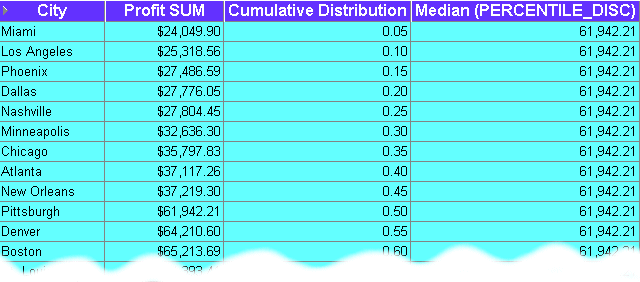
The worksheet shows the median profit value for cities. The median profit value (i.e. 0.50 in the Cumulative Distribution column) is $61,942,21 (i.e. the value for Pittsburgh, which has the value 0.50 in the Cumulative Distribution column).
Notes
On table worksheets, the calculation displays the returned value for each row in the worksheet. To return a single value, move the calculation into the Page Items area.
This example computes the median profit value for cities using the PERCENTILE_CONT function as a reporting aggregate function.
| Worksheet options | Set to: |
|---|---|
| Items | Video Analysis Information: City, Profit SUM |
| Sort Order | Not applicable |
| Conditions | Not applicable |
| Calculation Name | Median (PERCENTILE_CONT) |
| Calculation | PERCENTILE_CONT(0.5) WITHIN GROUP(ORDER BY Profit SUM) OVER() |
Figure A-28 Worksheet containing the Median(PERCENTILE_CONT) calculation
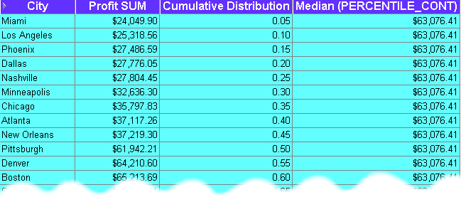
The worksheet shows the median profit value for cities. The median profit value is $63,076.41, which is the average profit value for the 0.50 and 0.55 percentile. In other words, the value for Pittsburgh plus the value for Denver, divided to two ($61,942.21 + $64,210.60)/2. For more information about how this function is calculated, see "About differences between PERCENTILE_CONT and PERCENTILE_DISC".
Notes
If the number of rows in the calculation is even, the two middle results are averaged. In the example above, the values for the .50 and .55 percentile are averaged.
On table worksheets, the calculation displays the returned value for each row in the worksheet. To return a single value, move the calculation into the Page Items area.
You use hypothetical rank and distribution functions for 'what-if?' analysis. These functions work out the position of a value if the value was inserted into a set of other values. For example, where would a person who generated sales of $1,200,000 be positioned in a ranked list of sales peoples' performance.
Note: You can also calculate the hypothetical values of the following:
DENSE_RANK - computes the rank of values where equal values receive the same rank (e.g. you can have more than one value ranked as top of the league)
CUME _DIST - computes the relative position of a specified value in a group of values
PERCENT_RANK - similar to CUME_DIST, this function calculates the rank of a value minus 1, divided by 1 less than the number of rows being evaluated
Examples:
This example calculates the hypothetical rank of profit values in relation to profit values for departments and regions. For example, to answer the question, how would a sales value of $500.00 be positioned in a ranked list of values for the Video Sale department in each region?
Note: This example uses a parameter to provide dynamic input to the calculation (for more information see "About using parameters to provide dynamic input to calculations").
| Worksheet options | Set to: |
|---|---|
| Items | Video Analysis Information: Calendar Year, Region, Department, Profit, Profit COUNT, Profit MAX, Profit MIN |
| Sort Order | Region (Lo to Hi) |
| Conditions | Not applicable |
| Page Items | Calendar Year=2000, Department=Video Sale, Value of Parameter Hypothetical Value=500 |
| Parameters | Hypothetical Value - this value is entered by the Discoverer user when the worksheet is opened or refreshed. |
| Calculation Name | League table |
| Calculation | RANK(:Hypothetical Value) WITHIN GROUP(ORDER BY Profit DESC NULLS FIRST) |
Figure A-29 Worksheet containing the League table calculation

The worksheet shows where the hypothetical value of $500 would rank in a ranked list of regions:
The hypothetical profit amount of $500 would rank number 2 in the Central region containing 520 profit values (range $13.49 to $537.78).
The hypothetical profit amount of $500 would rank number 7 in the East region containing 807 values (range $11.99 to $539.06).
Notice that because the hypothetical amount ($500) is greater than the Profit MAX amount in the West region ($484.01), the amount $500 has the hypothetical rank of number 1 for the West region.
Notes
The items Profit COUNT, Profit MAX, Profit MIN are not used in the calculation. They are displayed on the worksheet to help illustrate how the function is working. For example, if you can see that the Profit MAX value is $484.01 in the West region, you can see why a hypothetical value of $500.00 ranks as 1. This is because the hypothetical value is greater than the maximum value (i.e. the item Profit MAX).
The League table calculation uses the value of the :Hypothetical Value parameter, entered when the worksheet is opened or refreshed. In the example below, the Hypothetical Value (displayed in the Hypothetical amount page item) is set to 500. For more information about using parameter values in calculations, see "About using parameters to provide dynamic input to calculations".
The Rank function must take a non-aggregated value as an ORDER BY argument. For example, you could not perform this function on SUM(Profit) or Profit AVG.
As an alternative to setting the Hypothetical Value as a parameter, you could enter the rank value directly into the calculation as the Rank() argument. For example:
RANK(500) WITHIN GROUP(ORDER BY Profit DESC NULLS FIRST)
If you do not use a parameter, you will have to change the calculation to change the hypothetical value.
You use the Oracle9i WIDTH_BUCKET function to divide values into groups (sometimes called bands or buckets) according to their value (for more information, see "About banding"). For example, to group data for a bar graph.
Hint: You can also use the GREATEST and the CASE functions to calculate equi-width bands (see "Example: Banding by value (1)" and "Example: Banding by value (2)".
Examples:
This example divides profit figures into three bands according to their value.
| Worksheet options | Set to: |
|---|---|
| Items | Video Analysis Information: City, Profit SUM |
| Sort Order | Equi-width bands |
| Conditions | Department = Video Sale OR Department = Video Rental
Calendar Year = 2000 Region = Central |
| Calculation Name | Equi-width bands |
| Calculation | WIDTH_BUCKET(Profit SUM,0,30000,3) |
Figure A-30 Worksheet containing the Equi-width bands calculation
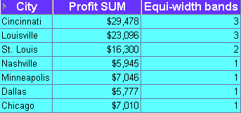
The worksheet shows equi-width bands for profit values for cities. The first band (0 to 9,999) contains Nashville, Minneapolis, Dallas, and Chicago. The second band (10,000 to 19,999) contains St. Louis. The third band (20,000 to 30,000) contains Cincinnati and Louisville.
Notes
The WIDTH_BUCKET function takes four arguments:
worksheet item = Profit SUM
minimum value = 0
maximum value = 30000
number of bands = 3
To assign bands in reverse order, reverse the minimum and maximum values. For example, WIDTH_BUCKET(Profit SUM,30000,0,3). This function produces the worksheet below.
Figure A-31 Worksheet containing the Equi-width bands calculation with reversed order
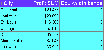
The worksheet shows equi-width bands for profit values for cities. The first band (20,000 to 30,000) contains Cincinnati and Louisville. The second band (10,000 to 19,999) contains St. Louis. The third band (0 to 9,999) contains Chicago, Dallas, Minneapolis, and Nashville.
You use FIRST/LAST aggregate functions to find the first or last value within an ordered group. This enables you to order data on one column but return another column. For example, to find the average sales transaction amount for the region with the largest number of sales transactions in a period.
Examples:
"Example: Find the largest sales transactions in area with most sales trans'"
"Example: Find the average sales transaction in area with least sales trans'"
Using FIRST/LAST functions maximizes Discoverer performance by avoiding the need to perform self-joins or sub-queries.
Note: You can use FIRST/LAST functions with the following:
MIN - find the smallest value in a list of values
MAX - find the largest value in a list of values
AVG - find the average value of a list of values
STDDEV - find the standard deviation of a list of values
VARIANCE - find the variance of a list of values
This example finds the largest sales transaction amount for the city with the most sales transactions in a period.
| Worksheet options | Set to: |
|---|---|
| Items | Video Analysis Information: City, Sales MAX, Sales Count |
| Sort Order | Not applicable
|
| Conditions | Department = Video Sale OR Department = Video Rental
Calendar Year = 2000 Region = Central |
| Calculation Name | Maximum sales in city with largest sales volume |
| Calculation | MAX(Sales MAX) KEEP(DENSE_RANK LAST ORDER BY Sales COUNT) OVER(PARTITION BY "Calendar Year", Region) |
Figure A-32 Worksheet containing the Maximum sales in city with largest sales volume calculation

The worksheet shows the largest sales transaction value in the city with the largest number of sales transactions. Cincinnati has the largest number of sales transactions (1220). The largest sales transaction for Cincinnati is $667.53.
Notes
Sales MAX - contains the largest sales transaction amount.
Sales COUNT - contains the number of sales transactions in the period.
To apply the function, Discoverer does the following:
orders the Sales COUNT column in the database (default order is ascending)
takes the last value in Sales COUNT column (i.e. the LAST argument), which is the largest number, and looks up the city name for this row (Cincinnati)
orders transactions in the database for Cincinnati and returns the LAST value, $667.53 (the default order is ascending)
The Sales COUNT and Sales MAX items are included to demonstrate that the calculation returns the correct result. The Sales COUNT and Sales MAX items are not used to calculate the result, which is calculated using aggregation in the database.
Hint: On table worksheets, the calculation displays the returned value for each row in the worksheet. To return a single value, move the calculation into the Page Items area.
This example calculates the average sales transaction amount for the city with the smallest number of sales transactions in a period.
| Worksheet options | Set to: |
|---|---|
| Items | Video Analysis Information: City, Sales COUNT, Sales AVG |
| Sort Order | Not applicable
|
| Conditions | Department = Video Sale OR Department = Video Rental
Region = Central Calendar Year = 2000 |
| Calculation Name | Average sales in city with smallest sales volume |
| Calculation | MIN(Sales AVG) KEEP(DENSE_RANK FIRST ORDER BY Sales COUNT) OVER(PARTITION BY "Calendar Year", Region) |
Figure A-33 Worksheet containing the Average sales in city with smallest sales volume calculation

The worksheet shows the average sales transaction value in the city with the smallest number of sales transactions. Nashville has the smallest number of transactions in the period (219). Therefore, the calculation returns the average transaction value for Nashville ($38.39).
Notes
Sales COUNT - contains the number of sales transaction in the period.
Sales AVG - contains the average sales transaction amount in the period.
To apply the function, Discoverer does the following:
orders the Sales COUNT column in the database (default order is ascending)
takes the first value in Sales COUNT column (i.e. the FIRST argument), which is the smallest number, and looks up the city name for this row (Nashville)
calculates the average sales value for Nashville, $38.39
The Sales COUNT and Sales AVG items are included to demonstrate that the calculation returns the correct result. The Sales COUNT and Sales AVG items are not used to calculate the result, which is calculated using aggregation in the database.
Hint: On table worksheets, the calculation displays the returned value for each row in the worksheet. To return a single value, move the calculation into the Page Items area.
The examples in this section show you how to use analytic functions with row-based and time-based intervals to get the best results with Discoverer. For example, you might was to create a calculation that returns the value of the previous row, or the value one year previously.
Note: Using row-based and time-based intervals is also known as windowing. For more information about windowing, see "About windowing". For more examples of using windowing in Discoverer, see "Windowing function examples".
The examples use analytic functions created using Discoverer's analytic functions templates. Each example shows how selecting intervals in the Restart calculation at each change in list on the analytic function template dialogs affects the calculation. For example, you might specify 1 Month Before Current Value as the interval, to compare sales in one month with sales in another month. For more information about creating calculation formulas using analytic function templates, see "How to create a new calculation using an analytic function template".
Note: If you are entering analytic function text in the Calculation field manually, you can specify an interval by adding a PARTITION BY clause to the formula. For more information about creating calculation formulas manually, see "What are analytic functions?".
This section contains the following examples:
"Example: Creating a Difference calculation using a row-based interval"
"Example: Creating a Difference calculation using a time-based interval"
"Example: Creating a Preceding value calculation using a time-based interval"
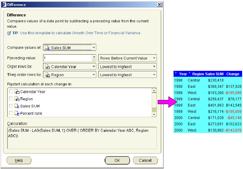
This example uses a difference calculation based on a row-based interval. The example worksheet displays the Year, Region, and Sales SUM items. To return the previous row's value for each sales value, add a calculation called 'Change' to the worksheet using the "Difference dialog", as follows:
select Sales SUM from the Compare values of drop down list
select the '1' and 'Rows Before Current Value' from the Preceding value fields
select 'Calendar Year' from the Order rows by field.
select 'Region' from the Then order rows by field.
accept default values for the remaining fields
The example worksheet shows the Change item containing the difference formula. For example, the Change column for the West region in 2000 is -$142,670. This value is derived from the West region value for 2000 (i.e. 130,982) minus the East region value for 2000 (i.e. 273,651).
Note: Positive values are shown in black. Negative values are shown in red.
Note: If you selected the Region check box in the Restart calculation at each change in list, you would always compare each value with the Sales SUM value for the same region in the previous year.
The example worksheet below shows the Change item containing the difference formula where the Region check box in the Restart calculation at each change in list is selected. In other words:
The Change value for the West region in 2000 is -$85,192. This value is derived from the Sales SUM value for the West region in 2000 (i.e. 130,982) minus the Sales SUM value for the West region in 1999 (i.e. 216.174).
The Change value for the East region in 2000 is -$128,331. This value is derived from the Sales SUM value for the East region in 2000 (i.e. 273,651) minus the Sales SUM value for the East region in 1999 (i.e. 401,983).
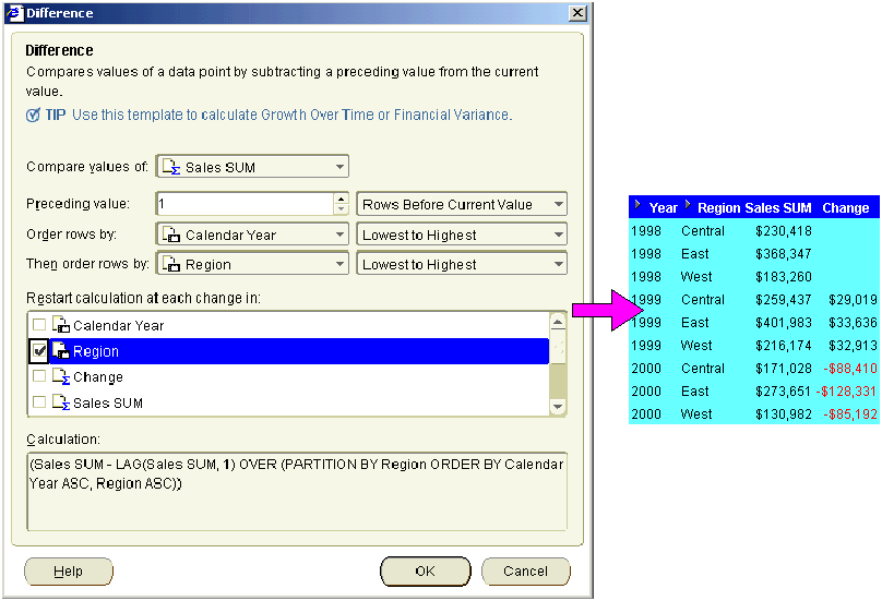
Note: When you choose a row-based interval and select the Region check box in the the Restart calculation at each change in list, you compare values with values from the previous year. You can also compare values with values from a previous year using a time-based interval (for more information about using time-based intervals, see "Example: Creating a Difference calculation using a time-based interval").
This example uses a difference calculation based on a time-based interval. The example worksheet displays the Year, Region, and Sales SUM items. To calculate the change in sales from the previous year, add a calculation called Yearly change to the worksheet using the "Difference dialog", as follows:
select Sales SUM from the Compare values of drop down list
select the '1' and 'Years Before Current Value' from the Preceding value fields
select the Region check box in the Restart calculation at each change in list
accept default values for the remaining fields
The example worksheet shows the Yearly change item containing the difference formula. For example, you can see in the Yearly change column that Sales SUM value for the West region in 2000 is $85,192 less that the West region in 1999.
Note: Positive values are shown in black. Negative values are shown in red.
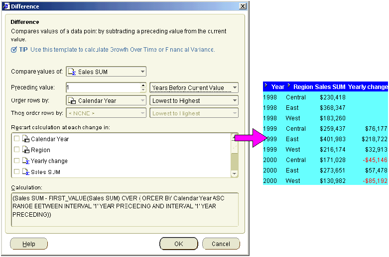
Note: If you did not select the Region check box in the Restart calculation at each change in list, you would always compare each value with the Sales SUM value for the last region in the previous year.
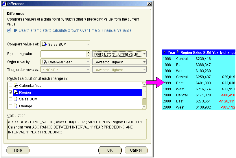
The example worksheet below shows the Yearly change item containing the preceding value formula where the Region check box in the Restart calculation at each change in list is cleared. In other words:
The Yearly change value for the West region in 2000 is -$85,192. This value is derived from the Sales SUM value for the West region in 2000 (i.e. 130,982) minus the Sales SUM value for the West region in 1999 (i.e. 216.174).
The Yearly change value for the East region in 2000 is $57,478. This value is derived from the Sales SUM value for the East region in 2000 (i.e. 273,651) minus the Sales SUM value for the West region in 1999 (i.e. 216.174).
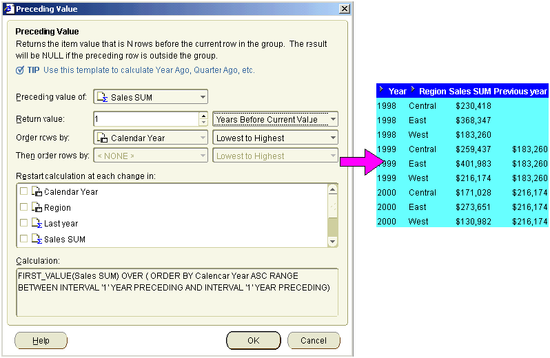
This example uses a preceding value calculation based on a time-based interval. The example worksheet displays the Year, Region, and Sales SUM items. To return the previous year's value for each sales value, add a calculation called Previous year to the worksheet using the "Preceding Value dialog", as follows:
select Sales SUM from the Preceding value of drop down list
select the '1' and 'Years Before Current Value' from the Return value fields
select the Region check box in the Restart calculation at each change in list
accept default values for the remaining fields
The example worksheet shows the Previous year item containing the preceding value formula. For example, you can see in the Previous year value for the West region in 2000 is $216,174, which is the same as the Sales SUM value for 1999 in the West region.
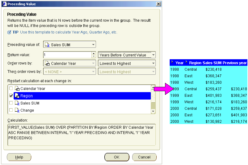
Note: If you did not select the Region check box in the Restart calculation at each change in list, you would always return the Sales SUM value for the last region in the previous year.
The example worksheet below shows the Previous year item containing the preceding value formula where the Region check box in the Restart calculation at each change in list is cleared. In other words, the Previous year value for the West, East, and Central regions in 2000 is $216,174, which is the same as the Sales SUM value for 1999 in the West region.
